Accelerated Excel Tricks (Part 1)

Whether you use Excel frequently or only once in awhile, it’s useful to discover tricks to help you quickly get the professional spreadsheet you’re after. Here are just 3 basics to easily make use of the program for your purposes.

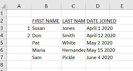
Sometimes you may have a list of data that is randomized, i.e. is not organized in order. Perhaps it’s a list of contacts you’ve been adding to as and when you receive them, but now you want to sort them in order and make presentable for sharing. Let’s use this simple unformatted list of names and dates to demonstrate a few shortcuts.

Adjusting Column Widths

First place your cursor at the right edge of the top row of the column you wish to adjust. The cursor will let you know you’re in the right position as the thick cross will turn into a thin cross with tiny arrows on the horizontal ends.

Let’s start with Column B that contains first names. You can either right click, hold and drag the column to the right to enlarge or to the left to shrink then release the cursor. Alternatively to let Excel decide the best width given all the contents of the column, instead of clicking and holding, simply double right-click once you’ve got the “thin” cursor. This is called auto-adjusting, and you can see below Column B now has its width set to incorporate the longest content (in this case the title).

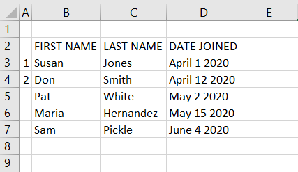
And now all column widths have been adjusted.

Adding to a Pattern

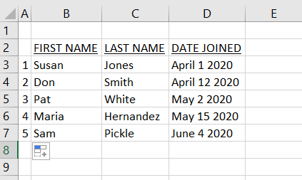
Excel allows you to start off a common pattern and issue a command to complete or repeat the pattern. This works for ordered numbers like lists and dates as well as days and months in words. In the above example, if we don’t want to have to fill in the numbers in the first column, we can use this feature. Simply highlight the pattern you have so far, place the cursor on the bottom right corner of the last entry until you get a solid cross (no arrows). Drag this down as far as you’d like the pattern to continue and release. You should get the pattern you intend. If you get something different, in this case say, 1,2,1,2,1,2 instead of 1,2,3, you’ll need to manually fill in more data before trying again.

If you need to add more rows later, you simply grab a few rows above the empty cells to establish the pattern (eg “3,4,5”), place the cursor again on the bottom right corner of the last number grabbed (“5”) then drag and release once you’ve covered all the cells you want. There is no need to grab from the beginning, just enough entries to establish the pattern.

Sorting your Data

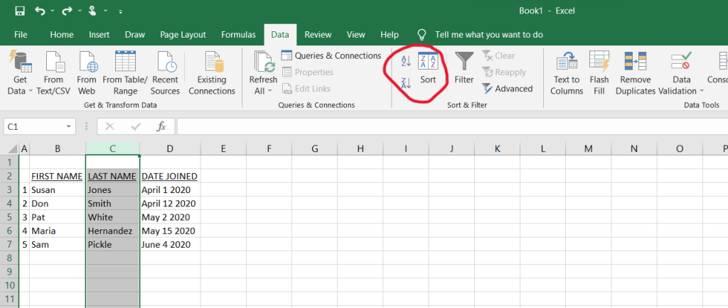
Excel will help you alphabetize any list or put in numerical order. In our example, say we now want to reconfigure the data alphabetically by last name. Click on the data in the column you want to sort (Last Name). In our example, you’ll click on the cell containing “C” above “Last Name”. Then click on the “Data” tab in your toolbar and look for the “Sort” option on the left. See below, left, with “Sort” circled in red.

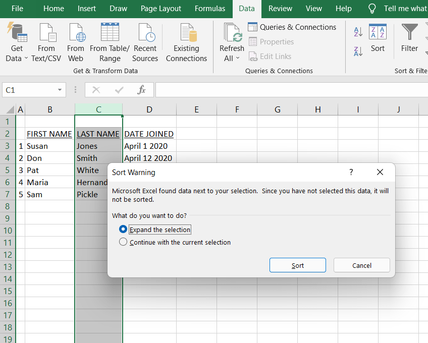
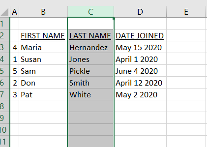
When the “A” is on top of the “Z,” that means your list will be sorted in alphabetical order. If this is the case, you just click on that button once. If however, the “Z” is on top of the “A,” you will need to click on the button twice. As you have now probably guessed, when the “Z” is on top of the “A,” your list will instead be sorted in reverse alphabetical order. Once you click “Sort” or “AZ”, in the case of our example, because there are related data (the first names corresponding to the last names), you will see the pop up message as above right. It is checking that you want to include the first names in the sorting exercise. Yes, we do. Otherwise we’d be jumbling people’s names and only sorting by last name. So keep the “Expand the selection” option ticked and click the “Sort” button at the bottom of the pop-up window. You can see below, we’ve now successfully sorted our list by last name.

Alternatively you can choose to sort by first name or any other column of data you find relevant. For example if you were compiling a list of donors to your charity or hours volunteered at your club, you might want to add a column of those numbers and sort by that in order to prioritize these contributors (or alternatively the laggards) in your communications or activities. You can always re-sort the data to alpha order when you’re finished with the analysis on donations.

Often we’ll want to maintain our data in more than one order. For example, we want the original list to be sorted by last name but maintain a copy of the list in another order (eg. joining date, contribution amounts, RSVP status, etc.). In this case, I suggest copying the original spreadsheet into a new tab and then re-sorting the copy. We’ll cover this in the very next blog, so be sure to subscribe if you don’t want to miss out.